Optimizing Streaming with Terrarium: Techniques and Insights

Overview

In my previous articles (Enhancing Streaming and Request Handling Efficiency with gRPC and Coroutines: Parts 3 and 4), I covered the general concepts behind request handling and streaming. However, every challenge calls for a customized solution. While coroutines can boost performance in some scenarios, they might also add unnecessary complexity, making the code harder to maintain without significant gains. Likewise, asynchronous streaming can sometimes underperform compared to synchronous methods if not implemented thoughtfully, often due to excessive context switching.

In this article, I’ll show how I optimized streaming algorithms in Terrarium to improve performance. I hope this approach can help you enhance your own implementations as well.

The problem

First, let’s clarify the goal. In Terrarium, streaming serves multiple purposes, but here I will focus specifically on implementing SQL support. The core idea is to use a virtual stream wrapper, where each streamer performs an operation and passes its result to the next streamer in the chain. In other words, streams are connected sequentially so that when a value is produced it flows through all streams until a final result is obtained.

To illustrate, consider the following example with a products table (Table 1):

Suppose we want to calculate the gross price of each product using the query:

SELECT 
ROUND(net_price * (1 + vat_percent / 100), 2) 
AS gross_price FROM products;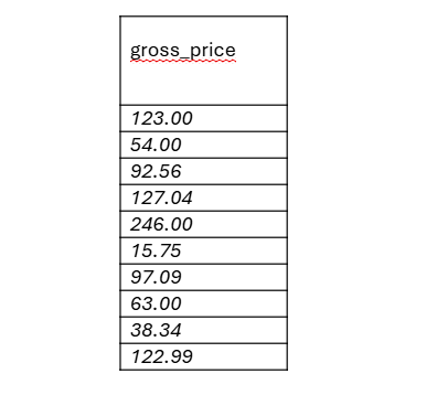 

The expected result is a single-column output of gross prices, as shown in Table 2. Now, let's examine how to chain streams to produce this result. After parsing, an Abstract Syntax Tree (AST) is generated and passed to the interpreter, which builds a chain of streamers. Each streamer performs a single operation and forwards its output to the next.

One initial approach is to organize streams in a tree structure (see Image 1). Starting from the root, calling operator() triggers recursive calls to other streamers until reaching the leaves, which terminate recursion and begin returning values.

For the calculation example:

1. Retrieve the vat_percent value from the table and divide it by 100.
2. Add 1 to the division result.
3. Multiply this sum by the net_price value from the table.
4. Round the final result to two decimal places.

This sequence requires eight streams: two of them fetch column values (vat_percent and net_price), while the others perform arithmetic operations without additional data access.

Since in Terrarium data is stored on worker nodes rather than on the gateway, any data retrieval requires querying these workers. To balance workload and prevent any single worker from becoming overloaded, we use sharding based on a shard key that determines how data is partitioned.

When fetching a column, we must query all workers (currently 2,160) to check if they hold the relevant data segment. Consequently, each table query involves opening 2,160 channels to collect the required data.

Using the streaming approach described earlier, the number of channels doubles—since two streams independently fetch data for net_price and vat_percent—resulting in 4,320 open channels.

This approach introduces several challenges:

• Excessive number of streams: We open more streams than necessary. Ideally, we should fetch all required data in a single call to avoid overwhelming the network layer.
• Inefficient data chunking: Streaming small chunks, such as fetching one column at a time, underutilizes the network. To maximize throughput, data should be sent in packets close to the MTU size (typically 1460 bytes).
• Limited parallelism: When calling operator() on a stream, data is fetched from only one worker at a time, leaving the remaining 2,159 workers idle. We need a strategy to collect data from all workers in parallel.
• Lack of callback support: The current recursive approach makes it difficult to integrate gRPC’s asynchronous callback mechanisms.
• Coroutines complexity: To leverage coroutines effectively, each stream would need to be rewritten as a coroutine, which can be challenging to implement consistently.
• Heterogeneous column types: Columns are stored as variants and can hold numbers, strings, maps, or other types. Since Terrarium supports schemaless data, columns may contain arbitrary data types.
• Memory management challenges: We want to process as much data in-memory as possible for speed, but handling very large datasets (e.g., 100 million rows) can exceed memory limits.
• JOIN operations: Fetching data from multiple tables adds further complexity, as data must be retrieved and combined efficiently across workers.
• And many more challenges beyond these.

In the following sections, I will explain how we redesigned the algorithm to improve streaming performance and address these challenges effectively.

Fetching data

When executing a query like SELECT * FROM table;, we create a single stream that fetches the entire row each time operator() is called. This is ideal because it allows us to handle data retrieval in a single call—exactly the behavior we want, even for more complex queries. However, users can specify more precise filters, such as:

SELECT * FROM table WHERE object_id = 8;  

SELECT * FROM table WHERE object_id IN (8, 10); 

If object_id is also the shard_key, we can calculate which worker holds the data. Instead of querying all 2,160 workers, we contact just one, significantly improving performance.

To support this, we need three types of data-fetching strategies:

• Broadcast stream – queries all workers.
• Worker stream – queries a specific worker.
• Partial broadcast stream – queries a subset of workers.

These can be unified under a single class with three methods:

• BuildStreamForAllWorkers();
• BuildStreamForAWorker();
• BuildStreamForAFewWorkers();

Each method builds the necessary streams based on the shard_key. The interpreter analyzes the query to identify all columns that need to be fetched, and then calls the appropriate method.

As shown in Image 2, instead of building a tree of streams, we construct a chain. Each stream instance knows in advance which columns to consume—for example, positions 0, 1. Based on how it's initialized. This design avoids creating multiple streams for each individual column. As a result:

• We reduce the number of open channels per worker.
• We minimize data transfer by avoiding redundant column fetching.
• We lower the number of stream object and operator() calls.

Another optimization relates to constant values. Previously, we streamed them for every row, even though they never change. A simple solution, which I implemented in the Round stream, involves storing constant values as class members instead of streaming them. Extending this approach to the Divide and Add streams can reduce memory usage on a per-row basis.

Of course, some queries do operate on two columns—for example:

SELECT net_price + vat_percent FROM table; 

To support both constants and column-based operands, I use a binary stream design that holds two std::optional<Variant> members. The logic is as follows:

• If the first variant is initialized (e.g., SELECT 10 + col1), it represents a constant; we only stream the second value.
• If the second is initialized (e.g., SELECT col1 + 20), we only stream the first value.
• If both are initialized (e.g., SELECT 10 + 20), the stream is computed entirely from constants—no data access required.

This design reduces the number of streamed columns, simplifies memory usage, and improves overall performance by reducing unnecessary computation and data transfer. ‍

‍

‍

Optimizing Data Chunk Size

When streaming a single column—such as a numeric value—we often transmit only a few bytes per row. This is highly inefficient, especially considering that a typical Maximum Transmission Unit (MTU) is 1,460 bytes. Sending small amounts of data per message significantly slows down streaming. To avoid this, we should aim to send data in chunks that approach or exceed the MTU. While calculating the exact size of each row at runtime may be inefficient, we can approximate chunk sizes or adopt a fixed-row batching strategy—for example, streaming 20 to 30 rows per chunk. This ensures each read operation transmits enough data to make efficient use of the network. Even if the last packet is not completely filled, the overall throughput is much higher. For example, streaming 30 rows totaling 21,700 bytes results in 14 full MTUs and a final partial packet with 1,260 bytes. This is far more efficient than sending individual 723-byte messages.

In another case, if each row is only 48 bytes, batching 30 rows yields 1,440 bytes, almost filling a single MTU. In contrast, sending 30 individual 48-byte packets introduces significant overhead—each TCP packet includes a header (~40 bytes), and each must be acknowledged, further reducing throughput. The table below shows a benchmark measuring streaming performance using asynchronous gRPC on a single thread. The test was run in our local environment:

As shown, performance increases dramatically with larger row sizes and fewer individual messages. Batching helps saturate the available bandwidth, reduces overhead from headers and acknowledgements, and minimizes context switches.

By carefully choosing chunk sizes and minimizing the number of small messages, we can significantly improve the efficiency of asynchronous gRPC streaming, especially under high-load conditions.

Parallelizing Stream Execution

Reading data from 2,160 workers using a single thread is highly inefficient. To speed up processing, we must utilize all available CPU cores. But how can we do this when each stream depends on the output of the previous one? For simple queries like:

SELECT * FROM table 

opportunities for parallelism are limited. The output is written directly to a socket, typically handled by a single thread. Even if we try to prefetch data sequentially using multiple threads, it won’t help in cases like ORDER BY, which requires globally sorted results. To address this, we need a different strategy. Instead of a single stream, we should open N parallel streams, where N equals the number of threads the CPU can handle. Each thread processes a portion of the data in parallel. Once data processing is complete, we can apply parallel-friendly algorithms (e.g., parallel sort, hash-based aggregation) to handle operations like ORDER BY, GROUP BY, and HAVING.

Let’s look at a more complex query:

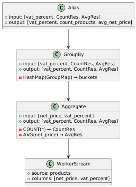
SELECT vat_percent, 
COUNT(*) AS count_products,
AVG(net_price) AS avg_net_price
FROM products GROUP BY vat_percent; 

In this case, we want to:

• Group rows by vat_percent (e.g., 5, 8, 23)
• Count how many products fall into each VAT group
• Calculate the average net_price for each group

Since data is distributed across all workers, we can process it in parallel by assigning different workers to different threads. For example, with 36 threads, each thread can handle responses from 60 workers (2160 / 36).

To avoid bottlenecks due to shared locking (e.g., using a single mutex), we introduce buckets to distribute access. Each thread maintains multiple buckets—say, 4 buckets per thread—to reduce competition. In this case, we’d have 144 buckets total (36 × 4).

Each incoming row is processed as follows:

By employing multiple worker streams and parallel threads, the volume of data fetched and reduced can be significantly increased compared to single-threaded processing. For instance, using 4 reading threads distributed across 16 workers results in substantial improvements in synchronous streaming performance, as illustrated in Table 4. The observed speedup ranges from approximately 75% to 160%, clearly demonstrating the benefits of parallelization. This improvement results from better CPU core utilization and more efficient network resource usage, enabling higher throughput and reduced latency.

Drawbacks of Asynchronous and Synchronous Streaming Approaches

In my previous articles, I encouraged implementing asynchronous request handling and streaming due to its potential speed advantages. However, this is not always the optimal choice in every scenario. In our case, the number of threads (e.g., 48 or 64) is significantly lower than the number of workers (2,160), making it infeasible to handle all worker responses concurrently. Although the gRPC interface supports callbacks for asynchronous response handling, our streams are implemented recursively, and adopting recursive callbacks would necessitate a comprehensive redesign, which we aim to avoid.

There are three alternatives:

• Coroutines: Rewriting all streams as coroutines would allow us to elegantly resume processing as soon as data becomes available. Coroutines provide clean, non-blocking flow control and avoid manual state management. However, the downside is the significant engineering effort required to retrofit every existing stream and callback into a coroutine-compatible structure—something that is both time-consuming and error-prone given our current codebase.
• std::promise / std::future: Another option is to use std::future in each stream to block on get() until the completion queue fulfills the corresponding std::promise. Once data is available, the promise is resolved, resuming the blocked thread. While easier to implement than full coroutine support, this method incurs additional context switching:
• A thread blocks on get(),
• Another thread sets the value in the completion queue,
• Then we re-block on the next Next() call for the next chunk.  This results in two thread switches per message, leading to inefficient CPU usage.
• Semaphores: it provides a lightweight synchronization mechanism that avoids constructing new promise/future pairs for every chunk. We can signal availability and resume the waiting thread with less overhead. However, semaphores still involve context switching (a thread waits, another signals), and do not fundamentally solve the latency introduced by frequent thread suspensions and resumptions.

Table 5 presents results for streaming large volumes of data from 2160 workers using 16 threads. As observed, the lower context-switching overhead in the synchronous method leads to faster streaming performance compared to the asynchronous approach—at least in scenarios where we are only fetching data without additional processing.

Moreover, when streaming such a large volume, the slower initialization phase of the synchronous method becomes relatively negligible. However, this advantage depends on the readiness of the workers. If workers take significantly longer to initialize, the asynchronous method may become more beneficial due to its ability to overlap initialization and data transfer.

Is it possible, then, to enable streaming in our current implementation without a major rewrite? Yes, by using synchronous streaming. In this approach, each call to the Read method blocks until a new row becomes available. Although this blocking mechanism is less efficient—since threads remain idle while waiting rather than processing responses concurrently—it offers a significantly simpler implementation within the constraints of our existing architecture.

Could we combine the benefits of both approaches to mitigate their drawbacks and achieve optimal performance?

1. Initialization Speed: Asynchronous streaming shines during initialization because it can start data collection in parallel across all 2160 workers. In contrast, synchronous streaming must wait for each worker to become ready sequentially, leading to longer startup times.
2. Context Switching Overhead: Asynchronous streaming incurs substantial context switching because completion queues and streams operate on multiple threads. Each new event requires resuming the appropriate stream, often causing expensive thread switches. Coroutines reduce thread switches but still require managing coroutine states. Synchronous streaming blocks until data is ready, eliminating the need for separate threads managing completion queues and reducing context switch overhead.

To illustrate these trade-offs, Table 6 presents a benchmark comparing both methods on a smaller dataset, where worker initialization time has a more significant impact on the total streaming duration. The results highlight that excessive context switching in asynchronous streaming reduces overall throughput. The "Total Time" column reflects the full duration of the streaming process, including worker initialization, while the "Read Time" isolates the performance once all workers are ready and data transfer begins.

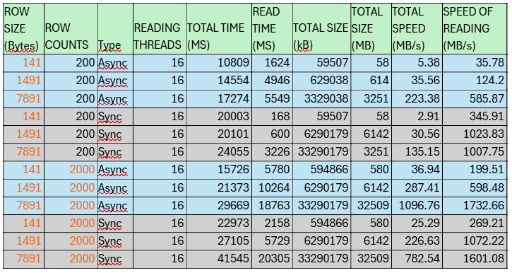
We observe that the asynchronous version exhibits significantly lower Speed of Reading, sometimes even up to 10 times slower than the synchronous approach. However, when comparing total times, the asynchronous method is only about 2 times slower for smaller chunks (e.g., 141 bytes) and around 50% slower for larger chunks. This difference stems from the fact that synchronous streaming spends most of its time initializing all 2160 workers sequentially, whereas asynchronous streaming initializes them quickly but suffers from overhead due to frequent context switching.

To leverage the strengths of both approaches, we propose a hybrid streaming method:

• Each streamer internally uses the asynchronous method to initiate and handle streams independently.
• Crucially, streams do not share a common completion queue, eliminating the need for a dedicated thread to manage event tags and thus drastically reducing costly thread context switches.
• During initialization, we concurrently trigger all worker streams and wait until each signals readiness by advancing their individual completion queues.
• Once all workers are ready, fetching rows is performed by directly calling Next on each worker’s completion queue — akin to synchronous reads but without invoking the Read method on the stream object itself.

This hybrid approach merges the fast parallel initialization of asynchronous streaming with the minimal context-switching overhead of synchronous reading. By avoiding shared completion queues and enabling direct, thread-local access to stream events, it effectively eliminates the major performance bottlenecks of both models.

As a result, the system achieves superior end-to-end throughput, especially under high concurrency, where traditional synchronous streaming would stall during worker setup and asynchronous streaming would suffer from frequent context switches.

Table 7 presents benchmark results for this hybrid implementation. As shown, the hybrid version is not only faster than the asynchronous variant, but in many cases also outperforms synchronous streaming by several factors, particularly for larger message sizes and high parallelism.

Memory management Considerations

At the final stage of streaming optimization, memory efficiency becomes critical—especially when processing millions or hundreds of millions of rows. Poor memory management can lead to excessive consumption, triggering disk spill and dramatically reducing query performance. One of the key challenges we faced in Terrarium was the representation of aggregated data. Since aggregation can happen both on the gateway (for instance when we JOIN tables) and individual workers, we needed a flexible mechanism to distinguish between raw and pre-aggregated values and handle them accordingly. To maintain a uniform data interface, we treat every value as a variant, which may encapsulate different data types. When we receive pre-aggregated data from workers, we serialize it as a std::map<variant, variant>. For example, this JSON:

{ 
   "STD": 123.4 
   "AVG": 43.5 
   'COUNT" 34 
} 

is represented internally as:

• A variant containing a std::map
• Each map entry consists of a variant string key and a variant double or integer value

In contrast, for raw aggregates, we represent the data as a std::vector<variant>:

[123.4, 43.5, 34] 

This allows for more compact in-memory representation.

Memory Usage Breakdown On 64-bit architectures, common STL containers like std::string, std::map, and std::vector use approximately 24 bytes for metadata (e.g., size, capacity, pointer). A variant typically requires 32 bytes, due to alignment and type-discrimination overhead.

Pre-Aggregated (Map-Based) Representation:

• Map node overhead: 32 bytes (left, right, parent + color/alignment)
• Key (variant string): 32 bytes
• Value (variant double/int): 32 bytes
• Total per entry: ~96 bytes
• Total per map (3 entries): ~3 × 96 + 32 (variant as map container) = 320 bytes

Raw (Vector-Based) Representation:

• Vector container as variant: 32 bytes
• 3 × value variants: 3 × 32 = 96 bytes
• Total: 128 bytes

Impact at Scale

Assuming 3 aggregated values per row and 100 million rows, the difference is substantial:

• Pre-aggregated (map): 100M × 320 bytes = ~89.4 GB
• Raw (vector): 100M × 128 bytes = ~35.7 GB

This demonstrates a 60% reduction in memory usage by choosing a leaner internal structure. When operating at high scale, data representation isn't just a design decision—it’s a performance multiplier. By optimizing how we store and stream data, we prevent memory exhaustion, reduce cache pressure, and eliminate unnecessary allocations—ultimately enabling Terrarium to handle large-scale analytics efficiently.

Summary

In this article, we explored how Terrarium optimizes streaming by addressing key challenges such as excessive stream count, inefficient data chunking, limited parallelism, and complex asynchronous handling. By redesigning the streaming architecture to use chained streams with precise data fetching strategies and batching data into appropriately sized chunks, we significantly improved network utilization and throughput. Additionally, leveraging parallel processing across multiple worker nodes and threads allowed us to fully utilize available CPU resources while maintaining correctness in operations like GROUP BY and aggregation.

Finally, we demonstrated that a hybrid streaming approach—combining the fast initialization of asynchronous streaming with the low overhead of synchronous reads—offers the best performance in practice. This approach effectively minimizes context-switching costs while maximizing concurrency, leading to superior throughput and scalability.

These optimizations collectively enable Terrarium to efficiently process large distributed datasets, paving the way for more responsive and scalable SQL query handling over gRPC streams.

Mateusz Adamski, Senior C++ developer at Synerise